Explaining the option pricing model

Companies issuing stock as compensation or investment companies with equity interests in privately held companies are often required to determine the fair value of equity interests for compliance with IRC Section 409(A) regulations, stock compensation expense, or mark-to-market accounting.

For these companies or investors, the perception of the fair value of the most junior equity, called common stock, is often $0. This conclusion is based on the fact that there’s often not enough value left over for the common shareholders after accounting for paying debtholders and numerous rounds of preferred stock liquidation preferences. This viewpoint is based on assumptions derived from what is called the Current Value Method (CVM). This method utilizes what is called a “waterfall” approach, which allocates the total value of a company to the various classes of investors (i.e., debt, preferred and common stock, based on each class’s distribution rights in a hypothetical sale). However, while the common stock (or other classes) might not receive any proceeds in a hypothetical sale today, that is typically not the case in the future assuming the company achieves its goals.

Simply put, an offer for pennies on the dollar, to buy a class of stock with zero value from the current value method (waterfall), would likely be quickly rejected. That is because there is value in the stock’s claim on future value generation, which is akin to an option. This is why the option pricing model (OPM) is the preferred method for determining the value of all classes of equity across the capital structure (assuming there are no recent arm’s-length transactions). But what exactly is the OPM, and how does it work?

Let’s consider a simple capital structure:

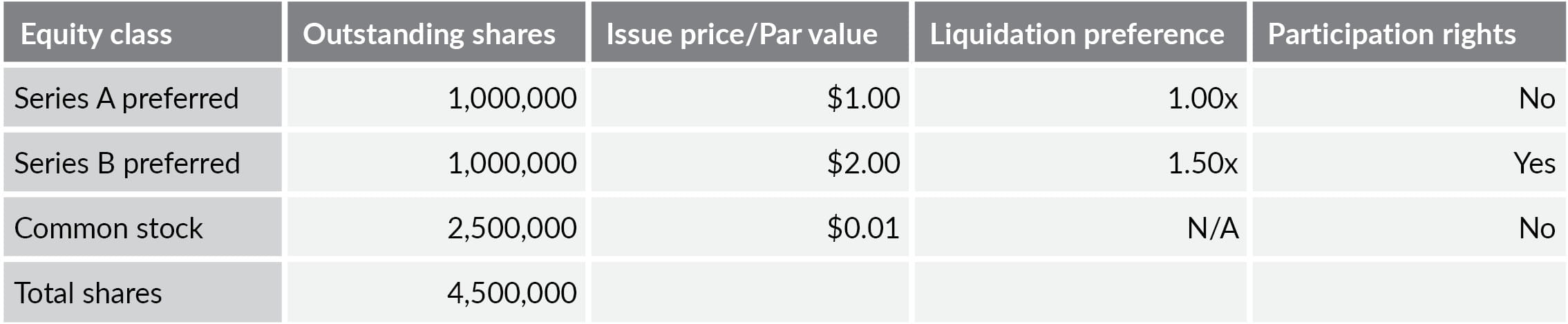
In the capital stack illustrated above, the total preferred liquidation preference is $4 million (Series A = 1,000,000 * $1.00/share and Series B = 1,000,000 * $3.00 ($2.00 * 1.5)/share). This is the amount owed to the Series A and Series B preferred stock in a liquidation event.

Let’s assume that the executive team determined the fair value of equity of the company is $2.5 million. With this fact pattern, under a hypothetical liquidation value of $2.5 million, the common stockholder(s) and series A preferred stockholder(s) would walk away empty handed ($2.5 million sales proceeds less $2.5 million payment to Series B preferred = $0 available for common stock and series A). However, this doesn’t mean that common stock and series A preferred stock shares would be given away or be sold for pennies on the dollar. Intuitively, there is still value for the stock, but it’s not realized in the current value waterfall.

The OPM values all classes of equity as a call option on the respective share of equity each class is entitled to. 

The OPM values all classes of equity as a call option on the respective share of equity each class is entitled to. In the example above, under the OPM, the value of common stock is quantified by treating the common stock as a call option on the equity value of the company. This approach recognizes that, while the common stock and series A preferred stock would not receive any distributions if the company were sold today, they still retain the right to distributions in the future should the company generate enough value to exceed the distribution rights of the more senior preferred equity. Viewing common stock this way, it is easy to see the parallels between a call option and the various classes of equity. But how does this work in practice?

In a real life scenario, the appraiser first determines the valuation breakpoints. These are equity values in which the allocation of proceeds in a hypothetical sale shifts from one class of equity to another. From our example above, assuming the Series B preferred stock is the most senior security, the first breakpoint would be $3 million, equal to the total liquidation preference of the Series B preferred stock. Any proceeds above this breakpoint would be allocated to the next in line; in this case, Series A investors. Once the breakpoints are quantified, they are then utilized as the strike price for each class of equity within the Black-Scholes model to determine the option value of each class of stock. Based on this example, the breakpoints for the three classes of equity would be as follows:

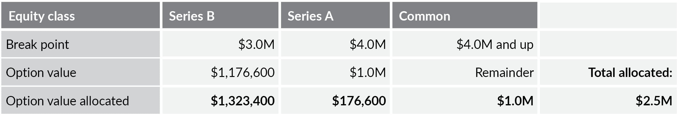
The option value allocated above to each class is not the total option value; it is the incremental option value. For Series B, the allocated value represents the value of a call option with a strike price of $0 and underlying value of $2.5 million (total equity value) less the value of the call option with a strike price of $3.0 million (Series B breakpoint). For Series A, the difference between the Series B and Series A option values is allocated. Finally, since there is no breakpoint at which another class of equity receives value, the Series A option value is allocated to common stock. The total allocation to all classes will always equal the total equity of the company; in this case it is $2.5 million.

Once the option value allocations are quantified, determining the per-share value is done by simply taking each class’s portion of each option value allocation and dividing by the number of shares outstanding. Note that since the Series B preferred has participation rights, the option value allocated to common stock would not go 100% to common stock; rather, it would go to common pro rata as if the Series B converted to common stock. In the example, 22% of the common stock allocation would go to Series B. To put it all together:

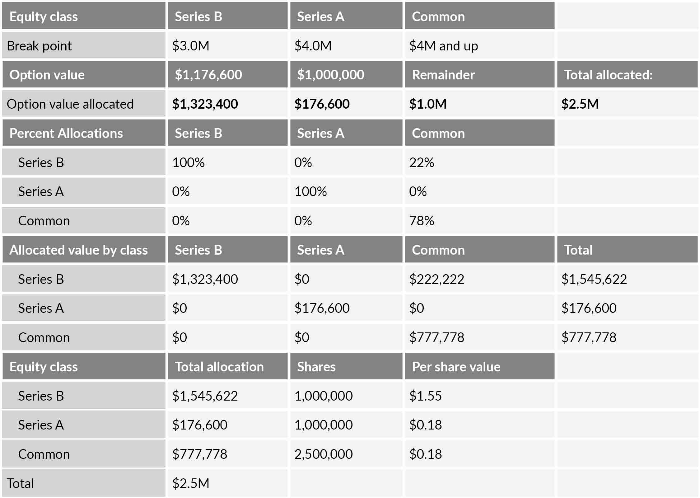
As you can see, the total value allocated to the common stock is $0.31 per share as opposed to $0 from the CVM. Also note that the Class A per share value is $0.18. Under the CVM, the waterfall would have allocated a $0 value to the Class A. Finally, the Class A value is lower than the common stock because the Class A total value potential is capped at the $1.0 million liquidation preference amount, while the common stock has unlimited upside.

The concluded per-share values would then be subject to a discount for lack of marketability, and an additional discount for lack of control would also be warranted. 

The concluded per-share values would then be subject to a discount for lack of marketability, and, if the bylaws or operating agreement of the company have control restrictions, an additional discount for lack of control would also be warranted.

Based on this illustration, it is easy to imagine how complex capital structures with numerous rounds of preferred stock, preferred warrants, and common options can generate a very complicated OPM model. However, it is a necessary part of the audit process for determining the fair value of various equity classes. Business owners, CFOs, and private equity investors often find that the engagement of a business valuation specialist can save considerable time not only with analysis but also with the audit process.